


The Policy Mosaic
An unstable policy equilibrium, IEEPA and degrees of freedom, soft data hardens, hard data softens, setting Fannie and Freddie loose

Unstable Policy Equilibrium
With Congress on recess and the President never taking a break, the market’s focus returned to trade policy after a couple of weeks of pressure on the back end of the Treasury yield curve as the One Big Beautiful Bill Act (1BBBA) advanced out of the House of Representatives. A month ago, we concluded we had passed peak policy pessimism, and the use of the International Emergency Economic Powers Act was likely to be ruled unconstitutional. The reaction in equities, fixed income and exchange rates to Liberation Day in early April had mitigated the risk of a 25% import consumption tax (tariffs), and the action of the Court of International Trade (CIT) modestly reduces that risk further. Last week our net takeaway from 1BBBA was it was a missed opportunity to put spending on track to reverse the Biden Budget Blowout (BBB), but the tax policy would not cause the deficit to widen, and the Treasury market would stabilize around 4.5% for nominal 10s, for the time being.
Stepping back and considering the policy mosaic, that is changes to tax, spending, regulatory, monetary, and trade policies, our view is the aggregate impact is favorable for equities, but less so for fixed income. The tax policy imbedded in 1BBBA is favorable for our outlook for a recovery in capital spending that if properly nurtured, could evolve into a secular boom that returns productivity growth to its longer run 2% trend after very tepid post-financial crisis growth. If Majority Leader Thune gets his way and the corporate investment tax expenditures on equipment, R&D and structures investment are made permanent, the probability of a secular boom like the ‘60s and ‘90s will increase further. Spending policy is improving modestly under 1BBBA, and there may be further progress during the annual appropriations process, but it remains unsustainably above the 20% level that will reduce net supply of Treasuries.
“The government spends like a drunken sailor, no, a drunken sailor spends his own money.” Jamie Dimon
Regulatory policy is progressing in the background, when Congress returns, they are likely to approve Federal Reserve Governor Bowman as Vice Chair for Bank Supervision, which is likely to lead to significant loosening of bank regulatory policy. Our checks with energy sector contacts indicate Secretary Wright is making significant progress, a critical underappreciated variable in the artificial intelligence investment boom, that is a crucial portion of our capex and productivity secular boom thesis.
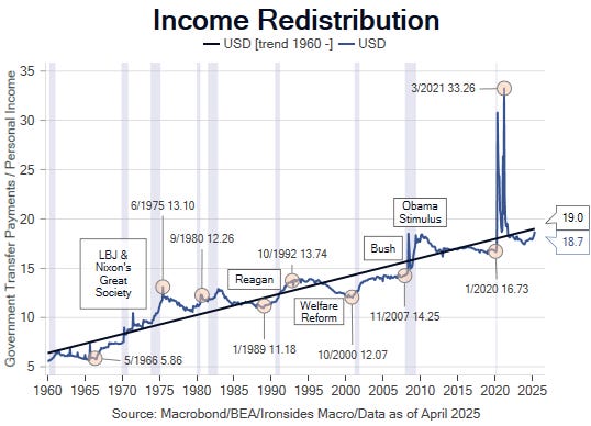
The outlook for monetary and trade policy are the biggest drags on the portion of the economy that is a potential Achilles Heel, the small business sector. During a call this week we were asked about our version of optimal Fed policy. In short, the Fed’s excessive pandemic policy response asset purchases misallocated capital to the benefit of asset-rich households, large banks and fixed rate investment grade borrowers, and their passive balance sheet contraction, combined with aggressive rate hikes tightening process shifted the majority of the burden of tighter policy to asset-lite households, small banks, real estate developers and small businesses. What they should be doing now is shortening the duration of their bond portfolio (reinvesting into bills) and reducing their policy rate by another 100bp.
Our answer about the degree of restrictiveness of the monetary policy setting is nuanced. Until the increase in the term premium and increase in long maturity real rates over the last 6 months, the balance sheet was providing accommodation for fixed rate borrowers. While that is less true today, if the Fed wants to lean against the largest inflation risk, they should reduce their holdings of longer maturity securities, thereby inducing reductions in government spending. Weak housing supply and small bank credit creation, due to weak profitability (low return on equity) strongly suggest the policy rate setting is restrictive. The probability of the FOMC adopting our policy suggestion is extremely low until there is a change in leadership in a year’s time, in the interim the pressure on the small business sector will persist. We recommend avoiding small caps.

Finally, that leaves trade policy, the subject of the next section of this week’s note.
Article 1, Section 8, Clause 1 & IEEPA
In our April 26 note, Peak Policy Pessimism, we discussed our view that Congress has transferred an excessive amount of discretion to federal agencies and the executive branch over a broad range of Constitutional responsibilities. We went on to conclude that the use of the International Emergencies Economic Powers Act (IEEPA) to enact tariffs was a violation of Article 1, Section 8, Clause 1 of the Constitution. On Wednesday, a 3-judge panel from Court for International Trade (CIT), appointed by Presidents Reagan, Obama and Trump, agreed with our conclusion. On Thursday, an Obama appointed judge to the DC District Court also ruled against the Trump administration’s use of IEEPA. The decisions, assuming they are upheld by the Supreme Court, and our interpretation of analysis from legal experts is the use of IEEPA is unconstitutional, do not derail the administration’s agenda. It does reduce their degrees of freedom to enact global tariffs, instead tariffs may need to be on specific products or countries. Unsurprisingly, the President increased the heat on China perhaps in response to the legal constraints.
Section 338 of the infamous Tariff Act of 1930 (Smoot Hawley) and Section 122 of the Trade Act of 1974 are the most sited alternatives to IEEPA. Section 338 allows the President to enact 50% tariffs on a nation discriminating against US commerce without an investigation, though it has never been used. Section 122 of the Trade Act of 1974 allows for 15% tariffs for 150 days in response to a growing current account deficit. In short, the CIT decision, and the actions of the Trump Administration following the market rejection of the trade surplus penalties (reciprocal tariffs), has taken the 25% tariff outcome off the table. This week’s events in no way derail the President’s trade agenda, but we now have less confidence in our base case of 10% global tariffs and 25-30% on China, the balance of risks is now skewed towards lower tariffs.
“Section 338 directs the President to impose tariffs “whenever he shall find as a fact” that a foreign country either (1) imposes on U.S. products “any unreasonable charge, exaction, regulation, or limitation which is not equally enforced upon the like articles of every foreign country” or (2) disadvantages and discriminates against U.S. commerce “by or in respect to any customs, tonnage, or port duty, fee, charge, exaction, classification, regulation, condition, restriction, or prohibition”—provided he finds that doing so will serve the public interest.”
Congressional and Presidential Authority to Impose Import Tariffs
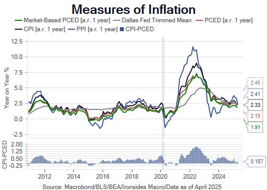
The administration is attempting to fast track the appeal process to the Supreme Court, consequently anything we write might have a limited half-life. That said, as we’ve discussed at length, tariff revenues were part of the fiscal plan. The potential loss of a portion of import consumption tax revenues does not change our outlook for the debt and deficit, in our view the only path to stabilization runs through returning spending to 20.3% of GDP. Of course, reduced tariffs, and increasing evidence that the aggregate effect is not inflationary, have (positive) implications for monetary policy as well.
(BN) FED'S GOOLSBEE: WITHOUT TARIFFS, INTEREST RATES COULD COME DOWN
Stabilizing Sentiment
The soft sentiment data got harder, and the hard activity got softer this week. Said differently, using an overly simplistic, overused euphemism, the soft data caught up to the hard data, and the hard data caught down to the soft data. Turns out the economy was not as ‘solid’ ahead of the Trump Trade Shock as FOMC participants would lead you to believe. The minutes of the May 6-7 FOMC meeting stated, “PDFP, which is often a better indicator than GDP of underlying economic momentum, rose at a solid pace in the first quarter”. The day after the minutes were released the advanced PDFP estimate of 3% was revised to a modestly less solid 2.5%. GDI was not included in the advanced estimate, in Thursday’s revision it matched the 0.2% contraction in GDP. The contraction was attributable to a sharp drop in the private sector net operating surplus, suggesting the front running of tariffs evident in the $163 billion increase in inventory investment, negatively impacted profit margins. Personal consumption expenditures were revised from a soft 1.8% quarterly annualized pace to an even softer 1.2%. The primary driver of soft consumption was services at 1.7%, down from 2.4%. The second estimate of GDP is even more stale than usual given the policy changes in 2Q, but it does weaken the Fed can afford to be patient narrative. The only area of strength was capital equipment information processing investment, perhaps stockpiling of data center equipment imports. The aggregate picture is disruption, FOMC participants characterization of final demand as solid is a stretch.
We also received some weak April activity data. The core capital goods component of the durable goods orders report contracted 1.3% from March and April pending home sales dropped 6.3% from March, on a quarterly basis the pending home index is at the lowest level in the 25-year history of this series. Finally, initial and continuing jobless claims for the weeks ending May 24 and 17 respectively increased more than expected to 240,000 and 1.919 million. For continuing claims this was the highest total since late 2021.

The last of the May Federal Reserve manufacturing and services surveys, as well as the Conference Board Consumer Confidence Survey, showed stabilization and recovery in manufacturing capital spending plans and consumer confidence. Labor market measures did not improve. There was evidence of increased tariffs negatively impacting services consumption and profit margins and capital spending in the services surveys underscoring the building evidence of spillover negative effects in the services sector from the import consumption tax (tariffs).

Manufacturing 6-month forward capital spending plans rebounded sharply to just below the January post-election peak. The divergence with service providing industries and technology capital spending plans is notable. The rebound in manufacturing was encouraging for our expectation of a capital investment recovery in 2H25, but the lack of confirmation from the larger services sector is concerning.

Another area of concern was the drop in prices received, even as prices paid remained at the April Trump Trade Shock high. The divergence is consistent with our view that the price elasticity of demand is high, in other words companies will struggle to pass increased costs through to the consumer. S&P 500 margins expanded in 1Q, but the national accounts GDI data suggests small businesses are struggling. Notably, the Cleveland Fed and Bloomberg Core CPI Tracking Estimates for May are 0.23% and 0.21% suggesting tariffs do not lead to higher consumer price inflation.
“The labor market was expected to weaken substantially, with the unemployment rate forecast moving above the staff’s estimate of its natural rate by the end of this year and remaining above the natural rate through 2027.”
Staff Economic Outlook, FOMC Minutes, May 7-8
While there was some modest recovery in 6-month forward employment plans in both the manufacturing and services surveys, the current readings for employment and hours worked remained near the expansion/contraction line suggesting demand for labor is soft.

No question the March and April employment reports were reasonably strong, however, the labor market data over the last month has been soft. In addition to the soft employment components of the Federal Reserve Bank surveys, and the aforementioned claims data, the May Conference Board Labor Differential was revised lower for April and slipped further in May to 13.2%, just above the September ‘24 12.7% reading before the Fed rate cuts and election-related improvement in business confidence. The 13.2% labor differential forecast for the U3 unemployment rate is 4.41% and 8.13% for the U6 underemployment rate, significantly higher than the April 4.19% and 7.8% levels. Due to the drop in immigration, the FOMC is likely to be more sensitive to increases in the unemployment rate than establishment survey employment growth. Governor Waller stated in a media interview that monthly increases of 0.2% or more in U3 would change his view that the labor market is solid. We will have more to say on the labor market in a preview note following the release of the April Job Openings & Labor Turnover Survey on Tuesday, but it looks like the risk is for a weaker than expected report.
The Return of Fannie and Freddie
The policy development overshadowed by trade policy this week was the potential public offerings of Fannie Mae and Freddie Mac equity. We couldn’t let this pass without a bit of a history lesson on these entities that were ground zero for the financial crisis. In 2002, during the deflation scare when Ben Bernanke made his infamous helicopter money speech, there was a refinancing boom that boosted the MBA Refi Index to nearly twice the pandemic peak. As a consequence, fixed income implied volatility spiked to historic levels, Freddie acted responsibly and continued to hedge their interest rate risk (convexity and duration), but Fannie Mae decided to run a massive speculative duration short of over $100 billion in 10-year equivalents. The markets sniffed it out, a massive squeeze resulted, Fannie lost ~$5 billion and Congressional hearings led to legislation and a new regulator, the FHFA.
With the implicit guarantee intact, the GSEs turned from interest rate risk to credit risk. From 2003 through 2008, the GSEs, along with other quasi-governmental agencies like the German Landesbanks, were the primary buyers of the super senior tranches of subprime collateral debt obligations. Those securities traded at extremely tight spreads, Libor plus 10-30bp, levels that only made sense with 60-70 turns of leverage that had an ancillary benefit of helping the GSEs meet their Community Reinvestment Act low-income housing requirements (turns out most of the loans were not in eligible low income MSAs but that’s another story). Without buyers for the super senior securities the subprime boom would not have reached its absurd end. In 2011 the FHFA sued the banking industry for $500 billion because their massive holdings of residential mortgage-backed securities (RMBS) were trading at 50, but ultimately the losses on the underlying loans were minimal, the hedge funds who bought the securities from the GSEs got rich, and the lawsuit faded after the government extracted massive fines from the banks.
If the GSEs are going to be returned to their prior status, we strongly suggest Congress pass legislation to shrink their footprint and expand the banking system’s role in the housing market. We would reduce the conforming loan limit and reverse Dodd Frank legislation that put excessive capital requirements on residential mortgage lending for banks. We would not leave this task to regulators that can be reversed with a change in administration or during the next recession. To be sure, without Fannie and Freddie, the 30-year fixed rate mortgage market, a product fairly unique to the US mortgage market, could not be nearly as large. It isn’t clear to us that the benefits outweigh the costs of the 30-year mortgage, homeownership in the US relative to economies with primarily floating rate mortgages is generally not higher. Additionally, the 30-year fixed rate mortgage makes monetary policy less efficacious. That said, classic economic liberals like us have been consistently disappointed since the financial crisis that the GSEs footprint in the housing market has grown despite their crucial role in the largest malinvestment bust in our 40-year career.
As to the securities, there are major questions about the amount of capital they will be required to hold, it should be on par with the banks, if not, the incentives to grow will inevitably lead to capital misallocation. There are lots of unanswered questions, we will have more to say if and when details develop.

Final Thoughts
We don’t see any obvious trades to lean into this week. Treasuries stabilized as we expected, the equity market rally from peak policy pessimism has stalled over the last couple of weeks. Over the next couple of weeks if we get weak labor market data and another round of cool inflation data, as well as the progress we expect on bank regulatory policy, there may be a case for increasing exposure to smaller banks and homebuilders.
We took a call from a Bloomberg reporter this week on our outlook for big tech following Nvidia’s results. In short, there was no pullback on artificial intelligence related capex. We have to agree with our friend Dan Ives; we are nowhere near the late innings of the artificial intelligence investment boom. The only drawback is the rich valuation of the sector, which makes it clear the trend is widely accepted. We prefer to lean into the infrastructure elements of the theme, but even with our very modest underweight in tech, our exposure is large.
We are a buyer of equities on weakness and a seller of fixed income on strength due to the broad policy mosaic. Within equities, consumer facing sectors margins are likely to be under pressure due to the import consumption tax, while industrials, technology, financials, materials and energy are likely to benefit from a recovery in capex. We will be watching the progress of 1BBBA in the Senate closely in the coming weeks.


Sector and Asset Allocation Tables Explained:
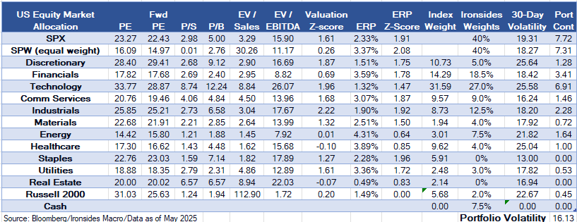
The US Equity Market Allocation table is our recommendations for a US equity investor, a similar approach to when we were the Head of Barclays US Equity Portfolio Strategy. The first six columns are valuation metrics, the seven is a Z-Score summary of the metrics relative to each sector’s valuation range since S&P introduced each sector (1990 for all but Real Estate). A reading of 1 implies the sector is 1 standard deviation above its historical median. The equity risk premium (ERP) column, also known as the Fed Model, is the forward (expected) earnings yield less the real 10-year yield (TIPS). Index weights are the S&P 500 with the exception of the Russell 200 small cap index, that is based on the market cap of the Russell 2000 relative to the Russell 3000. The final three columns are the Ironsides recommended weight, the 30-day volatility of the sector and portfolio contribution of our recommended weights to the risk (volatility) of the portfolio. Importantly, this approach does not integrate cross correlation of the sectors.
The asset allocation table benchmark is a 60/40 (stocks/bonds) portfolio, under the assumption that the investor is investing US dollars. We begin with our recommended weights, add the yield, the third columns are valuation metrics. ERP is the equity risk premium. TP is the term premium for Treasuries using the Adrian Crump & Moench model from Bloomberg. OAS is the option adjusted spread (early call risk) for fixed income securities. ‘SD’s’ from the median is a Z-Score approach to the valuation metrics, positive readings imply the asset is expensive, negative readings imply the asset’s valuation is below its longer-run median. The sixth column is the assets contribution to the risk of the portfolio, its volatility multiplied by the recommended weight of the asset. The index weights for equities use the same approach as the equity only portfolio, the fixed income weights are based on the Bloomberg US Aggregate Index, adjusted for the 60/40 benchmark. The final two columns are self-explanatory.
Barry C. Knapp
Managing Partner
Director of Research
Ironsides Macroeconomics LLC
908-821-7584
bcknapp@ironsidesmacro.com
https://www.linkedin.com/in/barry-c-knapp/
@barryknapp