The 10 Year Treasury Accord

The risk of a real rate shock is significantly reduced due to the actions of the Treasury Secretary Bessent and the FOMC reduction in QT

This week’s note analyzes the implications of the Federal Reserve's decision to reduce its quantitative tightening (QT) strategy, focusing on the potential impacts on liquidity, government spending, and monetary policy. We also provide an update on the economic soft patch and the market implications.

• QT Reduction Context: Chair Powell’s justification for the reduction of Treasury runoff from $25 billion to $5 billion per month was unconvincing, we suspect the administration's preferences played a significant role in this decision. There are significant market implications, in short, the FOMC eased policy.

• Policy Changes Under New Administration: Chair Powell’s listing of the new administration's policy shifts in trade, immigration, fiscal policy and regulation ordering may have been inadvertent, but our ranking of the relevant importance to investors would have almost completely reversed the order.

• Tariffs are Transitory: The Fed is correct to view tariffs as a transitory supply shock, unlike the pandemic policy panic there is not going to be a fiscal spending boom demand shock.

• Labor Market Dynamics: The collapse in labor market churn appears to be underappreciated by Chair Powell, we expect the unemployment rate to exceed the Fed's projections triggering a restart of the policy rate easing process.

• Corporate Tax Policy Outlook: Corporate tax reforms are in the works; these changes could positively influence private sector investment and economic growth and may explain decent industrials sector performance despite falling earnings revisions.

• Policy Outlook Stabilization: The Fed eased sooner than we expected, corporate tax policy is likely to begin to improve investor and the C-suite outlook. The least impactful in terms of gross domestic income, output, employment, capital spending and productivity of the administration’s ‘distinct’ changes to tax policy, spending, regulation, immigration and trade, is the one that has been the focus in recent weeks, trade.

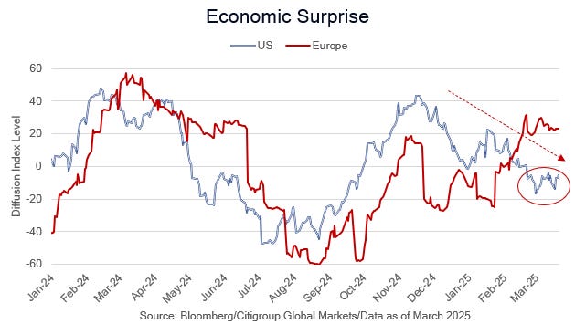
• The Soft Patch: Negative economic surprise has stabilized in recent weeks, however corporate results and policy sequencing and cleaning up the industrial policy mess (detox) suggest the soft patch is far from complete. We reached our downside equity market objective a week ago, but as a former colleague put it, ‘V’ bottoms are more the exception than the rule. There are sectors we would add exposure to including the belly of the Treasury curve.

The Curious QT Pivot & The 10-Year Treasury Accord

We are going to resist the temptation to dive into conditions in money markets and the Fed’s QT framework; suffice it to say, Chair Powell’s case for reducing Treasury runoff from $25 billion per month to $5 billion was weak. We were surprised by KC Fed President Schmid abandoning his third New Year’s resolution “to shrink the Fed’s footprint in financial markets”. Governor Waller’s dissent was consistent with our view that the liquidity framework detailed by the manager of system open market account (SOMA), Waller, Dallas Fed President Logan and Chair Powell was showing few signs of reserve tightness. We may be reading too much into Waller’s dissent, but if we are correct that the reduction in QT was a Treasury Secretary Bessent initiative, we suspect Waller took himself out of the running for Fed Chair. Finally, Governor Bowman also agreed to the reduction in QT, she likely has had extensive discussions with the administration’s economic team during their vetting of her for the Vice Chair for Bank Supervision role the President announced this week, consequently, her agreement, as well as the Treasury Secretary and President’s focus on 10-year Treasuries, suggests this is what the administration wanted. The above speculation about the motivation for the reduction in QT is consequential only in as much as it suggests the FOMC’s hurdle for resuming rate cuts may be closer than the press conference or post-meeting speeches implies.

“But in my view we are not there yet because reserve balances stand at over $3 trillion and this level is abundant. There is no evidence from money market indicators or my outreach conversations that the banking system is getting close to an ample level of reserves.”

Statement by Governor Christopher J. Waller

Figure 1: While the Treasury General Account (TGA) balance was falling due to the debt ceiling, bank reserves have been rising and are far from estimates of the lowest comfortable level. We define private sector liquidity as Fed assets owned outright less the TGA and the Fed’s reverse repo program balance, it has risen to the top of the post-rate hike range.

Whether there was an explicit agreement to stabilize the most important price in the global capital system while the US is Cleaning Up the Industrial Policy Mess (detoxing from the government spending addiction), and the Germans and Chinese are increasing government spending, the effect of reducing QT is significant. One way to frame this is to consider the US remains on track for another $2 trillion deficit (additional supply), with 2/3’s in notes and bonds, and without a reduction in QT the Fed was scheduled to reduce their holdings of Treasuries and mortgage-backed securities by an additional $500 billion. The reduction in QT will reduce Treasury net supply by $160 billion over the last 8 months of the year. We’ve now had Treasury Secretary Bessent decide to continue with former Secretary Yellen’s bill heavy issuance plans for at least two more quarters at his first quarterly refunding announcement (QRA), and the Fed reduce QT, as a consequence, real rates (TIPS yields) in the belly of the curve rallied sharply following the FOMC statement and 10-year real rates are 43bp below their mid-January peak.

Let’s be clear, we are not suggesting the decision to reduce QT is a threat to Fed independence. First, independence is a myth, as William McChesney Martin put, ‘the Fed is independent within, not of, the government.’ A ‘whole of government’ approach to debt management is crucial to the transition from the most accommodative fiscal policy in US history to a recovery in private sector capital spending. We remain convinced that until and unless federal government spending is returned to 20.5% of GDP, Treasury’s excessive bill issuance is cut, and the Fed’s balance sheet duration is shortened, Treasury investors will struggle to absorb the supply. Our view, prior to the 10-year Treasury Accord, was the path of least resistance for longer maturity Treasury yields was higher due to excessive supply and a loss of two decades of price insensitive buyers. The actions of the Bessent Treasury and Powell Fed are weakening the bias towards higher rates, but the real problem is government spending and even if the ‘big, beautiful reconciliation bill’ bends the spending curve, supply will remain high until the next fiscal year beginning in October. We’ve been recommending the belly of the curve (intermediate maturities), you may want to add some exposure if you are hiding out in the front-end (T-bill and chill).

Figure 2: This is the New York Fed’s measure of tightness in money markets, nothing to see here.

The Policy Mosaic

“Looking ahead new administration is in the process of implementing significant policy changes in four distinct areas, trade, immigration, fiscal policy and regulation. It is the net effect of these policy changes that will matter for the economy and for the path of monetary policy.” Chair Powell’s opening statement at Wednesday’s press conference

Perhaps Chair Powell’s list was in no particular order; that said, we would have changed and revised the list to government spending, tax policy, regulation, immigration and trade to prioritize impact of these policies on debt stabilization, capital spending, productivity, gross domestic income (GDI), output and inflation, in that order. As we’ve been explicit about, the focus on the first order effect on tariffs pales in comparison to the impact of reductions in government spending and delayed response of private sector investment to supply side corporate tax incentives and easier financial and energy sector regulatory policy. The Fed should be facilitating this transition, and while the Chair didn’t characterize the reduction in QT as a policy easing, less QT will help smooth this process on the margin. Additionally, condensing government spending and tax policy into a single category, fiscal policy, belies the new-Keynesian ideological bias of the FOMC and the staff, they tend not to differentiate between government and private sector spending. Powell amplified this bias in response to a question to a question about government employment growing faster than the private sector when he said, “from our standpoint, employment is
employment.”

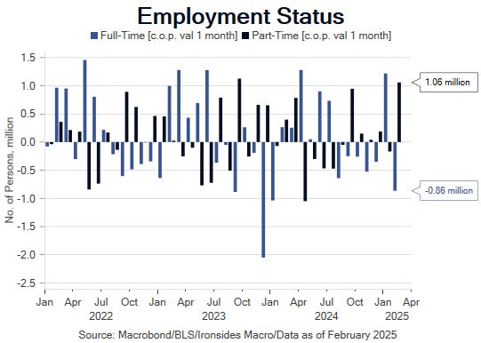
Finally, Chair Powell’s dismal of the collapse in labor market churn as “a low firing and low hiring situation”, underestimates the implications of low churn, namely lower real wage growth and productivity. Former NY Fed President Dudley, in a post-meeting Bloomberg interview put his finger on the crucial indicator that will determine whether the FOMC restarts the easing cycle, the unemployment rate. Lower immigration implies considerably slower monthly payroll gains, recall the composition of the ‘solid’ employment gains in February were 1.06 million part-time jobs and a loss of 860,000 full-time jobs. No reporter asked about the increase in the U6 underemployment rate (working part-time but would prefer full-time work) from 7.5% to 8.0%.

Figure 3: We do not understand anyone, policymakers in particular, with their army of economists, who characterize last month’s employment report as strong. Those who do are either lazy, uninformed or being disingenuous. If you want to call it an aberration, we can except that, though the actual aberrational reports were in September and January.

We are anxiously awaiting Tuesday’s March Conference Board Consumer Confidence for the labor differential. As we were drafting this note we received the LinkUp Monthly Jobs Recap, February 2025 Jobs Recap: The Labor Market froze up in February, stalled by Trump tariff chaos. The next round of labor market data is critical, the business confidence setback beginning in February due to policy sequencing and clumsy trade policy communication, government and contractor employment reversal, as well as the impact of the Fed’s pause on the yield curve, stalling the easing of financial conditions for floating rate borrowers, small banks and businesses, strongly suggest the unemployment rate is headed well above the Summary of Economic Projections (SEP) 4.4% year-end forecast.

Taken in its entirety, the FOMC meeting kept them on a path for a policy pivot to rate cuts despite the increase in SEP personal consumption deflator forecast from 2.5% to 2.7%, distribution of projections to higher inflation, and marginal increase in the DOT plot. On the other side of their stable price’s mandate, the median forecast for GDP went down and unemployment went up, with the risks skewed towards lower growth and higher unemployment. The 2s10s breakeven curve remains deeply inverted, as was the case in the months prior to the June ‘22 inflation peak, suggesting Chair Powell’s use of the word transitory was not the gotcha moment the press suggested. The big difference between the ‘21-’22 supply shock and an increase in tariffs in ‘25, also a supply shock, is that inflation is always and everywhere a fiscal and monetary phenomenon. Government spending is heading lower, consequently, higher tariffs remain a greater risk to personal consumption than the deflator.

Tax Policy: More Than Just an Extension

During the first 2 months of President Trump’s second term the equity market has focused primarily on the least important of the 5 major policy initiatives, trade, while the Treasury market’s emphasis has been titled towards the most important initiative, reduced government spending. In the background it appears progress is being made on corporate supply side tax reforms, an initiative crucial to both stocks and bonds due to the positive implications for private sector capital formation and productivity. We hear frequently there is little upside to extending the Tax Cuts & Jobs Acts, but we disagree, the Biden Administration and 117th Congress allowed key equipment and R&D investment provisions to expire, and capital investment slowed for the subsequent two years.

One of the big, albeit inside baseball, issues that appears to me evolving in a direction that will facilitate corporate supply side provisions is the use of current policy, rather than current law, as the baseline for the Byrd Rule constraint on bills passed under reconciliation. We will know with certainty in the next few weeks when the Senate passes their budget resolution if current policy is the baseline, our understanding is the Senate Budget Chair and Majority Leader are supportive, this leaves the Parliamentarian as the final hurdle. House budget hawks like the Freedom Caucus appear supportive as well, though that support is probably contingent on a minimum of $1.5 trillion of budget cuts (over 10 years).

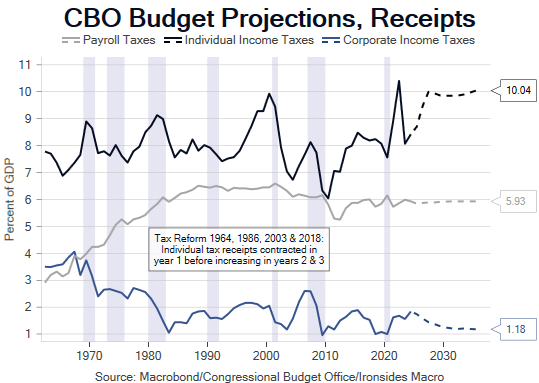
The logic in using current policy as the baseline is the history of the receipts to GDP ratio, as well as the impact of supply side tax reform on capital spending. As a reminder, the two biggest post-war capital spending booms in the ‘60s and ‘90s followed corporate tax rate cuts and increased investment provisions like those initiated early in the Kennedy Administration. As we’ve noted, the median receipts to GDP ratio since WWII is 17.1% with an 80bp standard deviation by administration. From 1947 to 1980 the median spending ratio is 17.6%, since 1981 it is 20.5%, but it increased to 24% over the last three years of the Biden Administration and is projected to drift towards 25% over the next 10 years. The most revealing statistic is the 2.6% standard deviation by post-war administration, highlighting the independent or exogenous nature of spending. Consequently, the Congressional Budget Office (CBO) projections on spending are far more accurate than receipts, as you can see in our next chart the CBO expects a big increase in revenues from the expiration of the top individual tax rate, history suggests Treasury will never realize the CBO’s forecast.

Figure 4: The corporate tax rate is permanent; the individual rate is set to expire. History suggests the CBO is overestimating individual receipts and underestimating corporate revenues.

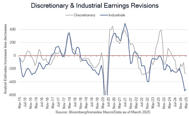
Following the passage of the Senate Budget Resolution we expect details of corporate tax provisions, immediate expensing of equipment and R&D investment and some form of accelerated depreciation for factory construction, to become more evident to investors. The work being done on these provisions may explain why the industrials sector has outperformed the S&P 500 year-to-date despite the deeply negative earnings revisions. In other words, there is no basis for analysts to increase estimates, but investor data dogs (reference explained in the next section) may have sniffed these tax provisions out.

Figure 5: Industrial sector revisions could bottom out; the consumer sector revisions may fall further.

Data Dogs

‘There’s a time for walking and a time for sniffing’ Chicago Fed President Goolsbee

Austan Goolsbee was a positive addition to the FOMC, if for no other reason than his entertaining and illuminating television interviews, we are not recommending him for Chair Powell’s job, but the press conferences would be more enjoyable. Sorry for the diversion, the previous sentence has nothing to do with this section other than we want to discuss what we learned this week about the progression of the economic soft patch, in other words, do some sniffing. The most important report of the week, February Retail Sales reported on Monday morning, lowered the Atlanta Fed Personal Consumption Expenditures (PCE) 1Q25 tracking model estimate from 1.1% to 0.4%, a level that is a major deceleration from 4.2% 4Q24 PCE. The details and anecdotal reports from Bank America’s CEO and Mastercard’s chief economist suggest the underlying trend create a more nuanced picture. In short, our skepticism of seasonal adjustment factors we discussed after the January retail sales report was supported by large swings in the ecommerce sales component, they were down 2.4% in January and rebounded 2.4% in February. Our view is that the 5% increase in ecommerce sales market share during the pandemic policy panic corrupted seasonal adjustment factors, consequently, the null hypothesis that consumption has slowed remains the most probable outcome, but the data is not conclusive.

Figure 6: The recent trend is towards the bottom of the range; the March report should provide a better reading on underlying demand as ‘silly seasonals’ wash out of the data.

This week’s housing data hinted at a nascent recovery, however, one month does not make a trend. Existing home sales rebounded but are captured when the sales close, consequently the data for February reflects demand in December and early January. The increase in both single and multi-family housing starts may reflect a thawing of the small and medium bank lending channel following the yield curve disinversion in 4Q24 and expectations of looser regulatory policy. The weekly bank lending data is picking up, it is running at a 4.3% annualized rate in 1Q25, a notable increase from 0.2% growth in 4Q24. On the other hand, the increase in starts may just reflect better weather from January’s polar vortex. The only other notable data this week, the March Empire State and Philly Fed manufacturing surveys, neither indicated a further deterioration in capital spending plans, nor a rebound. Next week we get the Richmond and Kansas City Fed surveys, and the S&P preliminary PMI surveys.

Notable corporate reports this week included Accenture’s struggles with their Federal Services division, the stock price and earnings call commentary suggest they been ‘DOGE’ed‘. The vast network of companies dependent on government spending is a risk to the labor market that is underappreciated by FOMC participants if we take their comments on the labor market at face value. Another notable earnings disappointment was FedEx, they attributed weak results to "Weakness in the industrial economy continued to pressure our higher margin B2B volumes. Similar to last quarter, this dynamic was most pronounced at freight, where fewer shipments and lower weights continue to negatively affect our results, albeit to a lesser extent than last quarter." This quote was provided by The Boock Report. FedEx beat on revenues, missed on earnings and cut capex, basically a poster child for trade policy disruption.

Next week’s data should be more illuminating than this week’s data, but the following week’s labor data is likely to prove more impactful. Manufacturing surveys will be helpful to quantify the magnitude of the business confidence setback. February Durable Goods Orders will provide additional ‘hard data’ on equipment investment. Frustratingly on Thursday we finally get 4Q24 gross domestic income, recall in 3Q24 GDI was much closer to potential growth at 2.1% than 3.1% GDP growth. Friday’s personal consumption, income and the deflator report is unlikely to provide any surprises.

Figure 7: The recent low in the Citi economic surprise index was February 28th, three weeks into March negative surprise has been stable in the marginally negative zone.

Market Wrap

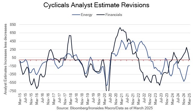
The two best performing sectors by some distance during the bounce off the 10% correction low has been energy and financials, our two tactical favorites due to the positive policy outlook. Net revisions are improving for energy, financials have given back the post-election positive momentum likely due to yield curve flattening and a slow start to capital markets activity. We expect to hear a considerable amount of policy loosening measures in the coming months and these two sectors are the two cheapest in our valuation framework. One quick note, forget about the price of crude, natural gas is a more important part of the US energy sector story. Additionally, our checks with energy strategists’ points to higher prices for crude if and when there is a truce in the Ukraine Russia war as an end to the price cap forces China and India to pay the market clearing price.

As to the broader market and the technology sector, we have two primary thoughts this week. First, paraphrasing our Macro Risk Advisors colleague John Kolovos, the Head of Technical Analysis, from a CNBC interview, ‘V’ bottoms are the exception, not the rule. The second related thought relates to fundamentals and the monetary policy response. For the FOMC to restart the cutting cycle, one way the equity market might be willing to look through the ‘detox’ process, the labor market, and consumer spending, will need to deteriorate further. If that occurs and the Fed does start cutting rates again in May or June, the first reaction might be positive, but most sustainable advances require positive earnings estimate momentum (revisions). As we detailed in this week’s note, the data didn’t get much worse over the last couple of weeks, however, the highest probability outcome is further deterioration. The 10-year Treasury Accord is reducing the discount rate for earnings, namely the real 10-year yield, but most of the market remains historically rich and 10-year TIPS at 1.9% are well above the ‘10s expansion range.

That said, the Fed eased sooner than we expected, corporate tax policy is likely to begin to improve investor and the C-suite outlook. The least impactful in terms of gross domestic income, output, employment, capital spending and productivity of the administration’s ‘distinct’ changes to tax policy, spending, regulation, immigration and trade, is the one that has been the focus in recent weeks, trade. We have to be incrementally more positive; policymakers are making progress in the detox process and as we wrote last week, despite trade policy communication missteps, we do believe the administration’s agenda remains on track.

Figure 8: These are the two biggest regulatory policy loosening beneficiaries. We expect revisions to pick up steam as earnings season approaches.

Sector and Asset Allocation Tables Explained:

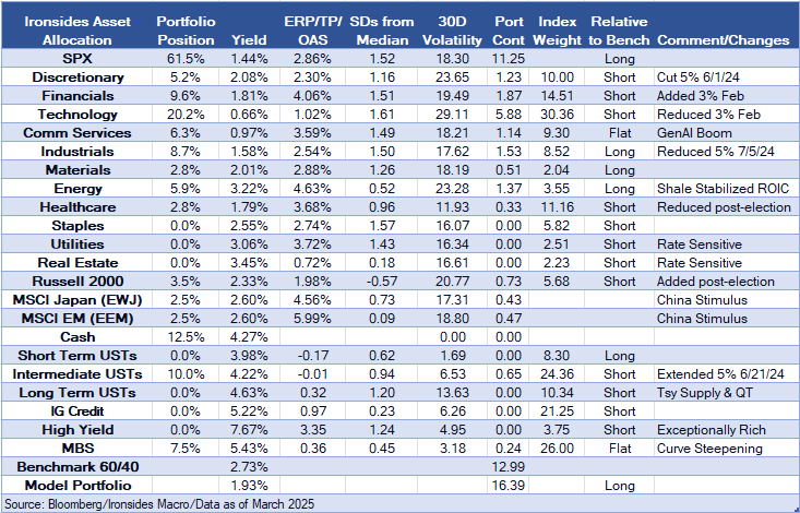
The US Equity Market Allocation table is our recommendations for a US equity investor, a similar approach to when we were the Head of Barclays US Equity Portfolio Strategy. The first six columns are valuation metrics, the seven is a Z-Score summary of the metrics relative to each sector’s valuation range since S&P introduced each sector (1990 for all but Real Estate). A reading of 1 implies the sector is 1 standard deviation above its historical median. The equity risk premium (ERP) column, also known as the Fed Model, is the forward (expected) earnings yield less the real 10-year yield (TIPS). Index weights are the S&P 500 with the exception of the Russell 200 small cap index, that is based on the market cap of the Russell 2000 relative to the Russell 3000. The final three columns are the Ironsides recommended weight, the 30-day volatility of the sector and portfolio contribution of our recommended weights to the risk (volatility) of the portfolio. Importantly, this approach does not integrate cross correlation of the sectors.

The asset allocation table benchmark is a 60/40 (stocks/bonds) portfolio, under the assumption that the investor is investing US dollars. We begin with our recommended weights, add the yield, the third columns are valuation metrics. ERP is the equity risk premium. TP is the term premium for Treasuries using the Adrian Crump & Moench model from Bloomberg. OAS is the option adjusted spread (early call risk) for fixed income securities. ‘SD’s’ from the median is a Z-Score approach to the valuation metrics, positive readings imply the asset is expensive, negative readings imply the asset’s valuation is below its longer-run median. The sixth column is the assets contribution to the risk of the portfolio, its volatility multiplied by the recommended weight of the asset. The index weights for equities use the same approach as the equity only portfolio, the fixed income weights are based on the Bloomberg US Aggregate Index, adjusted for the 60/40 benchmark. The final two columns are self-explanatory.

Barry C. Knapp

Managing Partner

Director of Research

Ironsides Macroeconomics LLC

908-821-7584

bcknapp@ironsidesmacro.com

https://www.linkedin.com/in/barry-c-knapp/

@barryknapp

This institutional communication has been prepared by Ironsides Macroeconomics LLC (“Ironsides Macroeconomics”) for your informational purposes only. This material is for illustration and discussion purposes only and are not intended to be, nor should they be construed as financial, legal, tax or investment advice and do not constitute an opinion or recommendation by Ironsides Macroeconomics. You should consult appropriate advisors concerning such matters. This material presents information through the date indicated, is only a guide to the author’s current expectations and is subject to revision by the author, though the author is under no obligation to do so. This material may contain commentary on: broad-based indices; economic, political, or market conditions; particular types of securities; and/or technical analysis concerning the demand and supply for a sector, index or industry based on trading volume and price. The views expressed herein are solely those of the author. This material should not be construed as a recommendation, or advice or an offer or solicitation with respect to the purchase or sale of any investment. The information in this report is not intended to provide a basis on which you could make an investment decision on any particular security or its issuer. This material is for sophisticated investors only. This document is intended for the recipient only and is not for distribution to anyone else or to the general public.

Certain information has been provided by and/or is based on third party sources and, although such information is believed to be reliable, no representation is made is made with respect to the accuracy, completeness or timeliness of such information. This information may be subject to change without notice. Ironsides Macroeconomics undertakes no obligation to maintain or update this material based on subsequent information and events or to provide you with any additional or supplemental information or any update to or correction of the information contained herein. Ironsides Macroeconomics, its officers, employees, affiliates and partners shall not be liable to any person in any way whatsoever for any losses, costs, or claims for your reliance on this material. Nothing herein is, or shall be relied on as, a promise or representation as to future performance. PAST PERFORMANCE IS NOT INDICATIVE OF FUTURE RESULTS.

Opinions expressed in this material may differ or be contrary to opinions expressed, or actions taken, by Ironsides Macroeconomics or its affiliates, or their respective officers, directors, or employees. In addition, any opinions and assumptions expressed herein are made as of the date of this communication and are subject to change and/or withdrawal without notice. Ironsides Macroeconomics or its affiliates may have positions in financial instruments mentioned, may have acquired such positions at prices no longer available, and may have interests different from or adverse to your interests or inconsistent with the advice herein. Ironsides Macroeconomics or its affiliates may advise issuers of financial instruments mentioned. No liability is accepted by Ironsides Macroeconomics, its officers, employees, affiliates or partners for any losses that may arise from any use of the information contained herein.

Any financial instruments mentioned herein are speculative in nature and may involve risk to principal and interest. Any prices or levels shown are either historical or purely indicative. This material does not take into account the particular investment objectives or financial circumstances, objectives or needs of any specific investor, and are not intended as recommendations of particular securities, investment products, or other financial products or strategies to particular clients. Securities, investment products, other financial products or strategies discussed herein may not be suitable for all investors. The recipient of this report must make its own independent decisions regarding any securities, investment products or other financial products mentioned herein.

The material should not be provided to any person in a jurisdiction where its provision or use would be contrary to local laws, rules or regulations. This material is not to be reproduced or redistributed to any other person or published in whole or in part for any purpose absent the written consent of Ironsides Macroeconomics.

© 2025 Ironsides Macroeconomics LLC.