


The Third Variable
Policy reflexivity, excess demand for autos, housing and labor, the Great Reallocation

Fed Policy Reflexivity
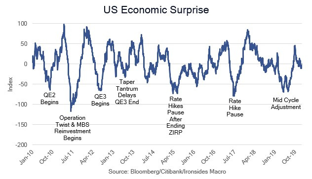
During the post-financial crisis period, household and financial sector deleveraging led to disinflation and lower nominal growth, an outcome that was predicted at the 2010 Jackson Hole Symposium by Carmen and Vincent Reinhart in After the Fall. Although they didn’t include disinflation in their key findings, almost as an addendum they described the disinflationary impulse following the post-WWII financial crises they studied as remarkable given the number that occurred in emerging market economies despite currency devaluations. As the US recovery progressed in fits and starts, investors became conditioned to focus on two variables: the growth outlook and monetary policy response. The combination of investor expectations (economic surprise) and lags in the Fed’s reaction function led to years (2010-2017) of growth scares followed by Fed easing just as the growth outlook was improving. The Fed’s normalization attempts, including the end of QE1 purchases and mortgage paydowns in 2010, the end of QE2 in 2011, scheduled end of Operation Twist in 2012, Taper Tantrum in 2013, end of QE3 in 2014, end of zero rates late 2015 and QT in 2018 were aborted not by inflation, but rather because of deterioration in the growth outlook.
Although it’s never different this time, it is rarely the same as last time. Enter the third variable this cycle, namely, inflation. The disinflationary ‘10s allowed the Fed to simplify their reaction function and turn their dual mandate emphasis to growth and employment. While the inflationary ‘20s has complicated the Fed’s reaction function, given the overriding Keynesian demand economic ideology of FOMC participants and staff, intractable inflation imbedded in expectations originates with demand for labor. Recall Larry Summers’ simplified inflation model: wage growth less productivity equals consumer price inflation. In the current environment, the Fed believes they can reduce surplus demand for labor (as we discussed in our note Payroll Preview: Productivity Dividend) and prevent longer-term market measures and consumer surveys from becoming unanchored from their target. Consequently, with goods inflation having peaked due to supply chains clearing and the appreciation of the dollar as well as house prices likely to peak due to the 220bp mortgage rate hike shock, a dynamic that will not be apparent in CPI or PCED for ~6 months, there is a window of at least three months where the Fed’s policy path is unlikely to change unless the growth outlook deteriorates and/or labor demand collapses. This implies 50bp hikes on June 15 and July 27, followed by 25bp on September 21 following the balance sheet contraction caps being raised to their maximum of $95 billion per month on September 1. The ‘taking a look around’ after front-end loading of rate hikes never meant a pause, it simply meant a slower pace of hikes as QT accelerated and they analyze outright sales of mortgages.